Kinematic Equations Explained with Examples and Tables

When I first began studying motion in physics, I realized that understanding how objects move is not just about watching them travel from one place to another. It is about describing that motion with clarity, precision, and mathematical relationships. Kinematic equations form the foundation of motion analysis in classical mechanics. They allow us to calculate displacement, velocity, time, and acceleration without worrying about the forces that cause motion. In this detailed guide, I will explain kinematic equations from the ground up, explore their derivations, applications, limitations, and provide structured tables to help you master them confidently.

What Is Kinematics?

Kinematics is a branch of mechanics that focuses on describing motion without considering the forces responsible for it. It answers questions such as:

• How far did the object travel?
• How fast is it moving?
• How long did it take?
• How quickly is its velocity changing?

Kinematics does not analyze why motion happens. That responsibility belongs to dynamics. Instead, it provides the mathematical framework to describe motion clearly and accurately.

Fundamental Quantities in Kinematics

Before exploring kinematic equations, we must understand the core quantities involved.

Displacement

Displacement refers to the change in position of an object. It is a vector quantity, meaning it has both magnitude and direction. Unlike distance, displacement considers direction.$$\text{Displacement} = \text{Final Position} – \text{Initial Position}$$Displacement=Final Position−Initial Position

Velocity

Velocity describes how quickly displacement changes with time. It is also a vector quantity.$$\text{Velocity} = \frac{\text{Displacement}}{\text{Time}}$$Velocity=TimeDisplacement​

There are two main types:

• Average velocity
• Instantaneous velocity

Acceleration

Acceleration measures how quickly velocity changes over time.$$\text{Acceleration} = \frac{\text{Change in Velocity}}{\text{Time}}$$Acceleration=TimeChange in Velocity​

Acceleration can occur when speed increases, decreases, or direction changes.

Time

Time is a scalar quantity that measures duration. It connects displacement, velocity, and acceleration.

Conditions for Using Kinematic Equations

Kinematic equations apply only under specific conditions:

1. Motion occurs in a straight line.
2. Acceleration remains constant.
3. Motion is analyzed in one dimension.

If acceleration changes or motion occurs in two or three dimensions with varying acceleration, more advanced calculus based approaches are required.

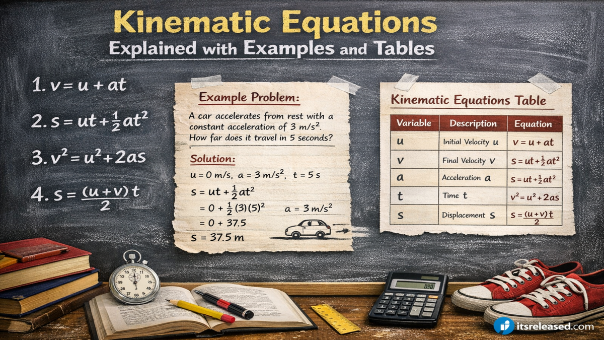
The Four Main Kinematic Equations

For constant acceleration motion in one dimension, we use four primary equations.

Equation 1: Final Velocity Formula

$$v = u + at$$v=u+at

Where:

Symbol	Meaning
v	Final velocity
u	Initial velocity
a	Acceleration
t	Time

This equation helps determine final velocity when acceleration and time are known.

Equation 2: Displacement Using Time

$$s = ut + \frac{1}{2}at^2$$s=ut+21​at2

Where:

Symbol	Meaning
s	Displacement
u	Initial velocity
a	Acceleration
t	Time

This formula calculates how far an object travels in a given time under constant acceleration.

Equation 3: Displacement Using Average Velocity

$$s = \frac{(u + v)}{2}t$$s=2(u+v)​t

This equation uses the concept of average velocity under constant acceleration.

Equation 4: Velocity Without Time

$$v^2 = u^2 + 2as$$v2=u2+2as

This formula is extremely useful when time is not given.

Summary Table of Kinematic Equations

Equation	Use Case	When to Use
v = u + at	Find final velocity	Time is known
s = ut + ½at²	Find displacement	Time is known
s = (u+v)/2 × t	Displacement with velocities	Both velocities known
v² = u² + 2as	Find velocity or displacement	Time not given

Derivation of Kinematic Equations

Understanding derivations strengthens conceptual clarity.

Deriving v = u + at

Acceleration is defined as:$$a = \frac{v – u}{t}$$a=tv−u​

Rearranging:$$v – u = at$$v−u=at$$v = u + at$$v=u+at

Deriving s = ut + ½at²

Velocity is displacement over time:$$v = \frac{s}{t}$$v=ts​

Since average velocity under constant acceleration equals:$$\frac{u + v}{2}$$2u+v​

Substitute v = u + at:$$\text{Average velocity} = \frac{u + (u+at)}{2}$$Average velocity=2u+(u+at)​$$= u + \frac{at}{2}$$=u+2at​

Multiply by time:$$s = ut + \frac{1}{2}at^2$$s=ut+21​at2

Types of Motion Covered by Kinematic Equations

Uniform Motion

When acceleration is zero:

• Velocity remains constant.
• Displacement formula simplifies to:

$$s = ut$$s=ut

Uniformly Accelerated Motion

Acceleration remains constant.

Examples:

• Free falling object
• Car accelerating at steady rate
• Object sliding down incline without friction change

Free Fall Motion

When objects fall under gravity alone:

Acceleration becomes:$$a = g$$a=g

On Earth:$$g \approx 9.8 \text{ m/s²}$$g≈9.8 m/s²

Kinematic equations remain the same but replace a with g.

Real Life Applications of Kinematic Equations

Automotive Industry

Engineers calculate braking distances using:$$v^2 = u^2 + 2as$$v2=u2+2as

This determines safe stopping distances.

Sports Science

Coaches analyze sprint acceleration and deceleration.

Aerospace Engineering

Rocket launch trajectories initially rely on kinematic motion equations.

Civil Engineering

Designing highways requires understanding acceleration lanes and stopping distances.

Graphical Interpretation of Motion

Position Time Graph

• Slope represents velocity.
• Curve indicates acceleration.

Velocity Time Graph

• Slope equals acceleration.
• Area under curve equals displacement.

Acceleration Time Graph

• Area under curve equals change in velocity.

Solving Numerical Problems Step by Step

Example 1: Car Acceleration

A car starts from rest and accelerates at 3 m/s² for 5 seconds.

Find final velocity and displacement.

Given:
u = 0
a = 3
t = 5

Final velocity:$$v = 0 + 3 \times 5 = 15 \text{ m/s}$$v=0+3×5=15 m/s

Displacement:$$s = 0 + \frac{1}{2}(3)(5^2)$$s=0+21​(3)(52)$$s = 37.5 \text{ m}$$s=37.5 m

Example 2: Braking Car

A car moving at 20 m/s stops over 40 meters. Find acceleration.$$0^2 = 20^2 + 2a(40)$$02=202+2a(40)$$0 = 400 + 80a$$0=400+80a$$a = -5 \text{ m/s²}$$a=−5 m/s²

Negative sign indicates deceleration.

Common Mistakes in Using Kinematic Equations

1. Ignoring direction signs.
2. Mixing units.
3. Using wrong equation for unknown variable.
4. Applying equations when acceleration is not constant.

Dimensional Consistency of Kinematic Equations

Each equation must maintain unit consistency.

Example:$$v = u + at$$v=u+at

Units:

m/s = m/s + (m/s² × s)

Units match correctly.

Comparison Between Distance and Displacement

Distance	Displacement
Scalar	Vector
Always positive	Can be positive or negative
Total path covered	Straight line change in position

Limitations of Kinematic Equations

• Cannot handle variable acceleration directly.
• Not suitable for rotational motion.
• Limited to inertial frames of reference.
• Does not include force analysis.

Extension to Two Dimensional Motion

Projectile motion uses kinematic equations separately for horizontal and vertical directions.

Horizontal:

Acceleration = 0

Vertical:

Acceleration = g

Importance in Academic Curriculum

Kinematic equations build the base for:

• Newton laws of motion
• Work energy theorem
• Circular motion
• Advanced mechanics

Students who master these equations find later physics topics easier.

Practical Strategy to Choose Correct Equation

Known Variables	Missing Variable	Recommended Equation
u, a, t	v	v = u + at
u, a, t	s	s = ut + ½at²
u, v, t	s	s = (u+v)/2 × t
u, a, s	v	v² = u² + 2as

Why Kinematic Equations Matter

Kinematic equations transform motion into predictable mathematical relationships. They allow engineers, scientists, and students to analyze real world motion without directly observing every detail. From calculating falling time of an object to estimating vehicle stopping distance, these equations are essential tools in physics.

Understanding them deeply strengthens logical thinking, analytical skills, and problem solving ability.

Conclusion

When I reflect on the importance of kinematic equations, I see them as the language of motion in classical physics. They allow us to quantify how objects move and predict future motion accurately. By mastering the relationships between displacement, velocity, acceleration, and time, one builds a powerful foundation in physics. Whether solving classroom problems or designing advanced mechanical systems, these equations remain indispensable tools in understanding the mechanics of our universe.

Click Here For More Blog Posts!

---

FAQs

1. What are kinematic equations used for?

They describe motion under constant acceleration without analyzing forces.

2. Can kinematic equations be used for circular motion?

No, they apply primarily to straight line motion with constant acceleration.

3. What happens if acceleration is zero?

Motion becomes uniform, and displacement equals velocity multiplied by time.

4. Why is acceleration negative in braking problems?

Negative acceleration indicates deceleration or motion opposite to chosen direction.

5. Are kinematic equations valid in space?

Yes, as long as acceleration remains constant and motion is in an inertial frame.